
| The Normal Distribution |
Continuous Distributions
The Binomial and Poisson distributions are discrete -- for they are based on counting successes rather than measuring data like a continuous distribution does. In other words, the data values are frequencies rather than measures. For example, if we're counting the number of customers in a grocery store who buy the ice cream that's on special, we would label a "buy" as a success and we'd build our probability distribution from the frequencies recorded. Obviously, frequencies are whole numbers since there's no such thing as "half a buy".
With a continuous distribution like the Normal distribution, our data comes from measuring things, such as the lengths of fish or the weight of a sample of bags of flour -- so the data values can be real numbers, not just integers, and they can take on a range of values between the minimum and maximum. With such distributions, we generally find the probability that a random variable will fall within a specific range or interval rather than equal a precise value. In a case where we want the probability that the random variable equals a precise and discrete value, we find the probability that it will fall between 0.5 below and 0.5 above that number.
So to find the probability that x = 4, we find P( 3.5 < x < 4.5) which is the probability that x is between 3.5 and 4.5.
The probabilities that result from a discrete distribution are often represented by a histogram. For continuous distributions, we use a continuous graph of the distribution function or probability density to represent the probabilities -- indicated by the area under the curve between the values in question. For such distributions, we rarely use the formula for the function. Instead, we use tables or calculators.
IMPORTANT NOTE:
not everyone has the same fonts, so if you see "r" and/or "l" in formulas,
change "r" to sigma  and change "l" to mu (µ)
The Normal Distribution
Characteristics of a Normal Probability Distribution:
The data in a normal distribution ranges from  . When we inspect the Normal Distribution Tables, we generally don't find a value of z greater than 3.09 and a z-value tells us the number of standard deviations between the data value and the mean.
The STANDARD Normal Probability Distribution:
This distribution is an exponential function determined by µ and  .
.
 is the function rule.
Using Intergral Calculus, we can prove that the area under this curve between negative and positive infinity is exactly = 1, therefore it can serve as a probability density function. However, to find values for the area under the cuve, we use the Normal Distribution table rather than integration. The values in the table tell us the probability of falling between the mean and the z-value in question.
P (z) = the probability of falling between µ and z in the belly of the distribution.
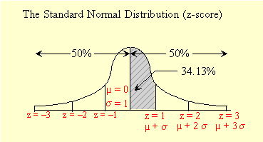
The values for z in the Normal Distribution Table tell us the probability of being in the zone between the given z-value and the mean µ. The shaded area in the diagram is P (0 < z < 1).
![]()
Finding Probabilities for Values of z:
When we look up the probability for z = 1 in the table, we find 0.3413. This means that 34.13% of the population falls between the mean and 1 standard deviation on either side of it. Had we wanted the probability that z < 1, we would add 0.5 to 0.3413 since now we include the 50% probability of being left of µ . If we needed the probability that z > 1, we would subtract 0.3413 from 0.5000, to get the probability of the tail. Drawing a diagram usually helps.
Example: Use the Normal Table to find:
Solution:
 ...... b)
c) 
![]()
Finding Values of z for Given Probabilities:
Say we know the z-scores of the students in a graduating class and we want to identify the top 10% to present them with certificates of merit. We would need to know what z-value cuts off 40% in the belly of the distribution since we need a top-tail of 10% and that leaves 40% between z and the mean.
When we look at the table, we find that a z of 1.28 gives a probability of 0.3997 and a z of 1.29 gives a probability of 0.4015 -- either of these will do, but if we really want to be picky and precise, we'd use z = 1.282 after some interpolation. We would then find the names of all students in the class with a z-score greater than 1.282.
Example: Find z if the standard-normal-curve area
Solution:
 ...... ...... b)
a) since we don't know if z is left or right of µ, the correct answer is z = ± 1.92.
b) since 0.9868 > 0.5000, we know the left half of the distribution is included, therefore the z-value must be right of the mean.We look up (0.9868 – 0.5000) = 0.4868. z = 2.22.
![]()
Z - or Standard score: (standardizing and comparing data values)
In order to compare data values from different populations or samples, we standardize the data and compare their z-scores.
Since z measures the number of standard deviations
between the data value x, and the mean l

with µ = population mean and  = population standard deviation.
Look at the formula.
The numerator ( x – µ ), is the distance between the data x-value and µ, the mean.
When we divide by  , we find how many of them there are in this interval.
![]() for a sample;
for a sample;  for a population
If z is negative, the data value is below the mean.
If z is positive, the data value is above the mean.
Using these formulas we can also solve for x and/or µ.

_____________________________
Example: Which is the better mark:
A) 89% in a class with mean 72%, standard deviation 9% or
B) 89% in a class with mean 72%, standard deviation 8.5%?
Solution: We find the z value for both.
A) (89 – 72)/ 9 = 1.89
B) (89 – 72)/ 8.5 = 2
The first mark is 1.89 standard deviations above the mean,
but the second mark is 2 standard deviations above the mean so it is the better mark.
_____________________________
Example: A biologist collects 20 samples of monster moths to record data about their enormous wing span. She measures in meters and her data indicate a mean wing span of 2.23 meters with a standard deviation of 0.42 meters. (these are steroid moths!!)
 's below the mean?
Solution:
 ) + l, in this case, x = – 0.23(0.42) + 2.23 = 2.13 meters
 ) + l, we find x = ( – 2.79)(0.42) + 2.23 = 1.06 meters
![]()
Practice
Make a diagram for all parts of #1 and #2.
1) Find the standard-normal curve area which lies:
| a) between z = 0 and z = 0.87 | b) between z = – 1.66 & z = 0 | c) right of z = 0.48 |
| d) right of z = – 0.27 | e) left of z = 1.30 | f) left of z = – 0.79 |
| g) between z = 0.55 & z = 1.12 | h) between z = – 1.05 & z = – 1.75 | i) left of z = – 0.15 |
| j) between z = – 1.95 & z = 0.44 | table |
2) Find z if the standard-normal-curve area
| a) left of z = 0.3085 | b) between – z and z = 0.8502 | c) between 0 and z = 0.4306 |
| d) right of z = 0.7704 | e) right of z = 0.1314 | f) between – z and z = 0.9700 |
3) Julie, Mark and Karen are in a class of 33 students. Their teacher gave them this data about their final marks in math:
| Student | Mark | Z-score |
| Julie | 60 | – 1.7 |
| Mark | 97 | 2 |
| Karen | 80 | ? |
4) Find the value of a, b, c and d.
| xi | l |  |
z |
| 12 | a | 2.5 | 1.6 |
| 30 | 26 | b | 1.3 |
| c | 12 | 1.2 | – 1.6 |
| 22 | 25 | 3.5 | d |
![]()
Solutions
1)
 ............... b)
 ............ d)
 ............f)
 ......... h)
 ................... j)
2)
 ..................b)
 ................d)
 ........0........ h)
3) Use 2 equations in l and 

 = 10. So Karen's z-score is 0.3
4) using the formula like in #3, find:
| a = 8 | b = 3.08 | c = 10.08 | d = - 0.86 |
![]()

(all content © MathRoom Learning Service; 2004 - ).
Normal Distribution Probabilities (Z-scores)
| Z | 0.00 | 0.01 | 0.02 | 0.03 | 0.04 | 0.05 | 0.06 | 0.07 | 0.08 | 0.09 |
| 0.0 | 0.0000 | 0.0040 | 0.0080 | 0.0120 | 0.0160 | 0.0199 | 0.0239 | 0.0279 | 0.0319 | 0.0359 |
| 0.1 | 0.0398 | 0.0438 | 0.0478 | 0.0517 | 0.0557 | 0.0596 | 0.0636 | 0.0675 | 0.0714 | 0.0753 |
| 0.2 | 0.0793 | 0.0832 | 0.0871 | 0.0910 | 0.0948 | 0.0987 | 0.1026 | 0.1064 | 0.1103 | 0.1141 |
| 0.3 | 0.1179 | 0.1217 | 0.1255 | 0.1293 | 0.1331 | 0.1368 | 0.1406 | 0.1443 | 0.1480 | 0.1517 |
| 0.4 | 0.1554 | 0.1591 | 0.1628 | 0.1664 | 0.1700 | 0.1736 | 0.1772 | 0.1808 | 0.1844 | 0.1879 |
| 0.5 | 0.1915 | 0.1950 | 0.1985 | 0.2019 | 0.2054 | 0.2088 | 0.2123 | 0.2157 | 0.2190 | 0.2224 |
| 0.6 | 0.2257 | 0.2291 | 0.2324 | 0.2357 | 0.2389 | 0.2422 | 0.2454 | 0.2486 | 0.2517 | 0.2549 |
| 0.7 | 0.2580 | 0.2611 | 0.2642 | 0.2673 | 0.2704 | 0.2734 | 0.2764 | 0.2794 | 0.2823 | 0.2852 |
| 0.8 | 0.2881 | 0.2910 | 0.2939 | 0.2967 | 0.2995 | 0.3023 | 0.3051 | 0.3078 | 0.3106 | 0.3133 |
| 0.9 | 0.3159 | 0.3186 | 0.3212 | 0.3238 | 0.3264 | 0.3289 | 0.3315 | 0.3340 | 0.3365 | 0.3389 |
| 1.0 | 0.3413 | 0.3438 | 0.3461 | 0.3485 | 0.3508 | 0.3531 | 0.3554 | 0.3577 | 0.3599 | 0.3621 |
| 1.1 | 0.3643 | 0.3665 | 0.3686 | 0.3708 | 0.3729 | 0.3749 | 0.3770 | 0.3790 | 0.3810 | 0.3830 |
| 1.2 | 0.3849 | 0.3869 | 0.3888 | 0.3907 | 0.3925 | 0.3944 | 0.3962 | 0.3980 | 0.3997 | 0.4015 |
| 1.3 | 0.4032 | 0.4049 | 0.4066 | 0.4082 | 0.4099 | 0.4115 | 0.4131 | 0.4147 | 0.4162 | 0.4177 |
| 1.4 | 0.4192 | 0.4207 | 0.4222 | 0.4236 | 0.4251 | 0.4265 | 0.4279 | 0.4292 | 0.4306 | 0.4319 |
| 1.5 | 0.4332 | 0.4345 | 0.4357 | 0.4370 | 0.4382 | 0.4394 | 0.4406 | 0.4418 | 0.4429 | 0.4441 |
| Z | 0.00 | 0.01 | 0.02 | 0.03 | 0.04 | 0.05 | 0.06 | 0.07 | 0.08 | 0.09 |
| 1.6 | 0.4452 | 0.4463 | 0.4474 | 0.4484 | 0.4495 | 0.4505 | 0.4515 | 0.4525 | 0.4535 | 0.4545 |
| 1.7 | 0.4554 | 0.4564 | 0.4573 | 0.4582 | 0.4591 | 0.4599 | 0.4608 | 0.4616 | 0.4625 | 0.4633 |
| 1.8 | 0.4641 | 0.4649 | 0.4656 | 0.4664 | 0.4671 | 0.4678 | 0.4686 | 0.4693 | 0.4699 | 0.4706 |
| 1.9 | 0.4713 | 0.4719 | 0.4726 | 0.4732 | 0.4738 | 0.4744 | 0.4750 | 0.4756 | 0.4761 | 0.4767 |
| 2.0 | 0.4772 | 0.4778 | 0.4783 | 0.4788 | 0.4793 | 0.4798 | 0.4803 | 0.4808 | 0.4812 | 0.4817 |
| 2.1 | 0.4821 | 0.4826 | 0.4830 | 0.4834 | 0.4838 | 0.4842 | 0.4846 | 0.4850 | 0.4854 | 0.4857 |
| 2.2 | 0.4861 | 0.4864 | 0.4868 | 0.4871 | 0.4875 | 0.4878 | 0.4881 | 0.4884 | 0.4887 | 0.4890 |
| 2.3 | 0.4893 | 0.4896 | 0.4898 | 0.4901 | 0.4904 | 0.4906 | 0.4909 | 0.4911 | 0.4913 | 0.4916 |
| 2.4 | 0.4918 | 0.4920 | 0.4922 | 0.4925 | 0.4927 | 0.4929 | 0.4931 | 0.4932 | 0.4934 | 0.4936 |
| 2.5 | 0.4938 | 0.4940 | 0.4941 | 0.4943 | 0.4945 | 0.4946 | 0.4948 | 0.4949 | 0.4951 | 0.4952 |
| 2.6 | 0.4953 | 0.4955 | 0.4956 | 0.4957 | 0.4959 | 0.4960 | 0.4961 | 0.4962 | 0.4963 | 0.4964 |
| 2.7 | 0.4965 | 0.4966 | 0.4967 | 0.4968 | 0.4969 | 0.4970 | 0.4971 | 0.4972 | 0.4973 | 0.4974 |
| 2.8 | 0.4974 | 0.4975 | 0.4976 | 0.4977 | 0.4977 | 0.4978 | 0.4979 | 0.4979 | 0.4980 | 0.4981 |
| 2.9 | 0.4981 | 0.4982 | 0.4982 | 0.4983 | 0.4984 | 0.4984 | 0.4985 | 0.4985 | 0.4986 | 0.4986 |
| 3.0 | 0.4987 | 0.4987 | 0.4987 | 0.4988 | 0.4988 | 0.4989 | 0.4989 | 0.4989 | 0.4990 | 0.4990 |
| Z | 0.00 | 0.01 | 0.02 | 0.03 | 0.04 | 0.05 | 0.06 | 0.07 | 0.08 | 0.09 |
.